Over the past few months, I've been preparing a guide with the tentative title, Excel for SEOs: Lessons for Aspiring Ninjas. I've embarked on this great journey because sometime during the #Mozinar back in September I decided that my Excel abilities were far too limited, especially compared to all the smarty pants that were giving great presentations and advice about SEO data analysis.

After talking with some of my colleagues I found that I wasn't alone in my feelings of Excel inadequacy. So Excel for SEOs: Lessons for Aspiring Ninjas was born as a means to help others by documenting my quest for Excel Ninj-ocity. The full document will be released sometime in January, but here is a selection that I hope provides some value alone.

Update: The guide has been released! Give it a read!

While having a working knowledge of the functions described below can help with a multitude of SEO tasks, the specific tasks that we'll be completing in the following include:

1. Isolating the root domains from a group of full URLs
2. Stripping the descriptive portion of a URL out of the full URL

-----SNIP-----

Lesson 2: More Functions - Text Manipulation

The functions on which we'll be focusing in this lesson are useful for dealing with text manipulation. As we'll see from the examples, there are quite a few scenarios wherein the SEO has to manipulate a text string. Some of the formulas we'll talk about are pretty simple to grasp individually, but can get a bit confusing when used together. We'll touch on:

• LEN
• SEARCH/FIND
• LEFT, RIGHT, MID

LEN

Microsoft Excel Definition: Returns the number of characters in a text string.

Syntax: LEN(text)

I doubt this requires much explanation. LEN alone is fairly useless. Sorry LEN.

SEARCH/FIND

Microsoft Excel Definition:
SEARCH - Returns the number of the character at which a specific character or text string is first found, reading left to right (not case-sensitive).
FIND - Returns the starting position of one text string within another text string. FIND is case-sensitive.

Syntax: SEARCH(find_text,within_text,start_num) and FIND(find_text,within_text,start_num)

There are two differences between SEARCH and FIND. SEARCH is not case-sensitive, FIND is. SEARCH allows the use of wildcards, FIND does not. Under most circumstances, SEARCH is all you need, but it helps to know that FIND is always there if you've got to deal with pesky capital letters in URLs or something similar. Another reason to choose FIND is if you're dealing with URLs that contain parameters. Without properly escaping question marks, they will act as wild cards, which may cause some frustration.

In our example below, we've pulled out the character number at which the "/blog/" string begins. Much like LEN, this function is a bit silly on its own, but can be combined with some of our other functions to do some cool things.

This is good but its not very pretty, let's use IFERROR to get rid of those #VALUE!s

The IFERROR syntax: IFERROR(value,value_if_error)

So much better!

LEFT, RIGHT, MID

Microsoft Excel Definition:
LEFT: Returns the specific number of characters from the start of a text string.
RIGHT: Returns the specific number of characters from the end of a text string.
MID: Returns the characters from the middle of a text string, given a starting position and length.

Syntax:
LEFT(text,num_chars)
RIGHT(text,num_chars)
MID(text,start_num,num_chars)

Both LEFT and RIGHT return the characters from a given position in a text string starting from either side of a string. MID is great for extracting a portion of a text string. I've lumped the three together because they are often used in conjunction with each other (along with a few of the earlier functions). Let's dive into an example:

Bringing it all together - Example 1

Let's say we've been given a list of URLs, and we want to extract just the domain.

This formula will do the job. Let's break down this nested formula, and see how it pulls just the domain out of our URL. Starting from the middle we see SEARCH, which uses the syntax:

SEARCH(find_text,within_text,start_num)

In plain terms, this formula finds the first instance of "/" in the cell to the left, starting at the 8th character from the beginning, which is done to start passed the double slash in http://. As we see below, the result for the first row of data is 22.

The same formula with the inner function calculated

Now we are left with a simple LEFT formula. Remember, the syntax for LEFT is LEFT(text,num_chars).

In plain terms: Give us the first 22 characters starting from the beginning. The number of characters differs depending on URL, but adjusts accordingly when applied to the rest of the table. We now have a nice listing of just root domains.

Our list of root domains. The formula reflects the change to a table format from the simple range used previously.

Example 2

Let’s use SEARCH (with wildcards) and MID together to extract a portion of a URL:

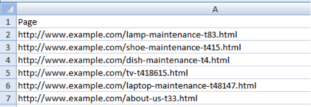
Let's assume we want to pull the descriptive piece out of each of these URLs for reporting purposes

We’ll definitely be making use of MID, as the text we want is in the MIDdle of our string. We’ll need to determine how many characters make up the "-tXXX.html" bit at the end of each URL. Since the length of this portion of the URL varies, but the format doesn’t (that is, "-t" + "numbers" + ".html"), we can use wildcards to find this character count.

Again, the syntaxes for these 2 functions:
MID(text,start_num,num_chars)
SEARCH(find_text,within_text,start_num)

Let's break down the formula for the first URL in our list.

Cell A2: http://www.example.com/lamp-maintenance-t83.html

=MID(A2,SEARCH("/",A2,8),SEARCH("-t*.html",A2)-SEARCH("/",A2,8))
=MID(A2,23, SEARCH("-t*.html",A2)-23)

We've calculated the first instance of a "/" after the 8th character. This gives us our start_num values. We're also using the * wildcard to help us get the character count of the right-most chunk of text.

=MID(A2,23,SEARCH("-t*.html",A2)-23)
=MID(A2,23,40-23)

We can easily calculate the number of characters for our MID once we know where our non-descriptive characters begin.

=MID(A2,23,17)
/lamp-maintenance

Hooray!

Example 2.5

Let's make a small adjustment to our original URL to demonstrate how we can use LEN in this formula.

Cell A2: http://www.example.com/t1521-lamp-maintenance.html

=MID(A2,SEARCH("-",A2)+1,LEN(A4)-SEARCH("-",A2)-5)
=MID(A2,29+1,50-29-5)
lamp-maintenance

The additional +1 and -5 are necessary to make minor adjustments to the final outcome. Without them, our final result would have been "-lamp-maintenance.html".

-----SNIP-----

Thus concludes the sample lesson on manipulating text strings in Excel. I hope you've found it useful, and not too confusing!

If you have any questions, ask away in the comments and follow me (@MikeCP) and @Distilled on Twitter for more info on the full release of Excel for SEOs: Lessons for Aspiring Ninjas. There's much more where this came from, including bits on pivot tables, VLOOKUP, Index/Match, OFFSET, and more!